Project 04 of 09
Machine Learning
Developing new ways to test a classification algorithm's predictability on new data.
- Context
- Leidos
- When
- Summer 2016
- Role
- Engineering intern
- Tags
- MATLAB, Python, Classification
 (image 1 of 19, view larger)
A Little Background
Machine learning is a buzzword nowadays, likely due to its resurgence and increasing prevalence in the media and academia during the past decade or so. Though the field is quite broad and most certainly multifaceted, you would not be doing yourself harm to interpret its meaning by exactly how it reads. Machine learning, in the loosest sense of the phrase, boils down to “teaching” a computer algorithm how to recognize and classify new data without continual supervision.
In this page I will provide a brief description of how the machine learning process generally works, outline the issues with current industry standards that I wish to address, and finally, the solutions that I came up with to overcome these problems.
Throughout my experiences with the subject, I have settled upon two pervasive questions which still linger in the field: What are the best strategies to tuning parameters of a learning algorithm, and further, how do I know that my algorithm actually has any predictive power on new data?
During the summer of 2016, the latter question was precisely the obstacle which I aimed to overcome.
To see just the final solution, skip to the very last section on the page.
The Industry Standard
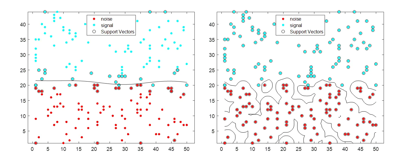
Cross Validation and the Holdout method are two of the most common methods of determining an algorithm’s test error. Explicitly, test error is the ratio of new data fed to the algorithm which it classified incorrectly. If this error rate is low, your algorithm is misclassifying a small percentage of the new data. This is ideal. There is another quantitative metric to determine an algorithms predictability on new data, and that is tune error. This is the ratio of points that the algorithm misclassified on the data used to train it. This is very important, and can be interpreted as how overfit your algorithm is on your training data. With one very small adjustment to the method by which this algorithm was trained, the difference in overfitting is easily illustrated below.
Underfit to the training data
Overfit to the training data
 (image 2 of 19, view larger)
This algorithm will likely generalize well when fed new data to test on. It seems to be the winner of the two in terms of capturing the true distribution of the data, not just where each of the points lie.
This algorithm will generalize very poorly to new data, as it has tuned to the training data far too much. It will likely classify a high percentage of new data from the same distributions incorrectly when tested on.
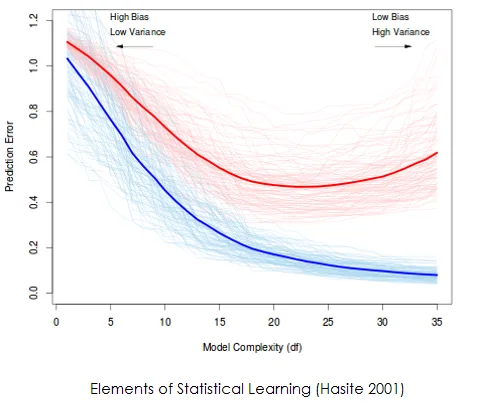
The graph on the right is a popular graph to illustrate the phenomenon above. For nearly all applications, a classification algorithm will be most desirable when it sits at the lowest point of the red curve in terms of complexity. At this point, the rate of misclassification for the algorithm on new data is the lowest (as per various methods of approximating test error), signifying the best "understanding" of the underlying distribution of the data.
 (image 3 of 19, view larger)
The blue curve is the misclassification rate on the training data. As the algorithm's complexity increases, it classifies fewer of these points incorrectly. As a consequence, it loses touch with the underlying distribution of the data, resulting in a higher and higher test error (red line).
 (image 4 of 19, view larger)
Closing in on the Issue
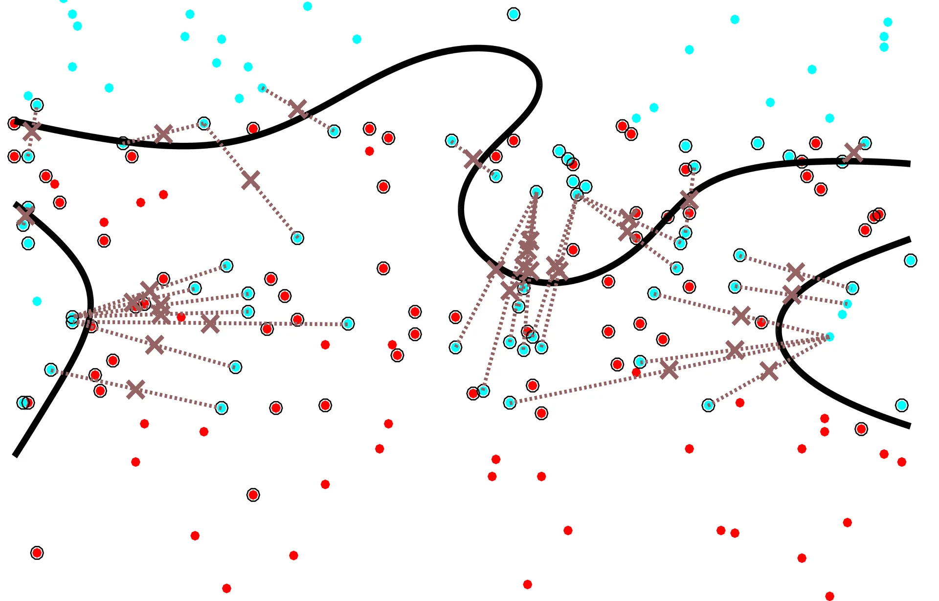
Now a large problem which arises in reality is that researchers do not have access to a continual supply of new data. In fact, access to new data is very uncommon. As such, researchers have developed ways of estimating this test error, to provide a quantitative measurement of how good an algorithm performs. There are issues I found unsettling with the two methods identified above which I attempted to mitigate through the development of new test error approximation algorithms. Briefly, the issues are described below.
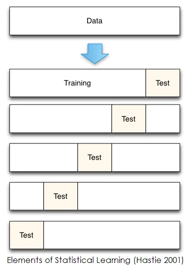
Cross validation and the holdout method, in short, hide a fraction of the sample data from the learning algorithm. Once a classifier is trained on the part of the sample data which is not hidden, the ratio of test error described above can be found by simply feeding the algorithm with the previously hidden data and analyzing the fraction of which it misclassified. The two major issues I find with cross-validation are that:
- The classifier that is built while measuring this test error through cross-validation is quite different from the one that the researcher will ultimately stick with, which has been trained on all of that data available, not just a fraction of it. The large assumption here is that the distribution represented by the fraction of the dataset is close enough to the actual distribution from which the data came. In certain data distributions, this assumption can be proven to be detrimental.
- Similar to the first point, if a researcher only has a very small amount of data to work with, let’s say, a cancer researcher. If he only has 6 known cases of a new cancer type to help identify the traits which give it away, should he really start dealing with fractions of this dataset? How could he be so sure that eliminating 1, 2, or even 3 data points are still going to provide a classifier which has a high predictive power?
 (image 5 of 19, view larger)
My Solutions
Perhaps the most exciting part of this project was that the work I was doing had very little established research to guide it. I took many shots in the dark, and watched almost all of them crash and burn as I soon figured out just how poorly they performed. The final solution that I came up upon was to create an algorithm which generates new data based off the traits of the available sample data, such that a trained classifier can be tested on this new data. This new data, if the algorithm is designed well, should be considered closely representative of the true distribution of the sample data. In this way, there is no data partitioning and thus probable misrepresentation of the true distribution of the data, and the entirety of the available data can confidently be used to train a learning algorithm.
It is worth noting that I did not come up with the idea of pseudo-data generation algorithms, but I came up with quite a few methods which fall into that broad category. Other established methods within this category that I experimented with included bootstrapping, kernel density estimation, and other forms of probability density fitting.
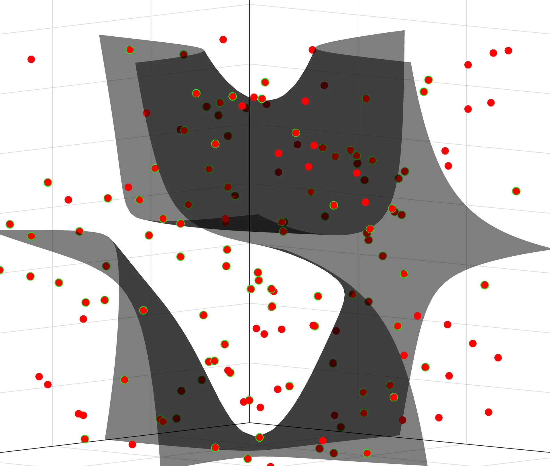 (image 6 of 19, view larger)
Methods
The first few methods I came up with were quite bad; and I will explain why. But going through each of these methods were very important stepping stones in guiding my thought progression to come up with my final algorithm, which performs extraordinarily well.
To start, I decided to try a simple interpolation scheme between points in the existing dataset in order to create a new set of data on which to test the algorithm’s efficacy. With this idea in mind, there were a few possible directions to go.
Firstly, I decided to focus on the decision boundary between classes in a sample data set. I chose to generate this new test set based on the points that the algorithm misclassified from the training set: a new point was to be generated at the Euclidean midpoint between every misclassified point in feature space and the nearest correctly classified point of the same class. The resulting point was then labeled as a member of this class, then fed into the algorithm to see if it got the label correct.
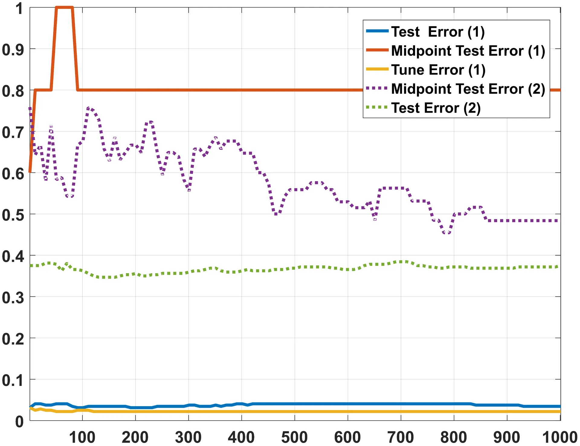
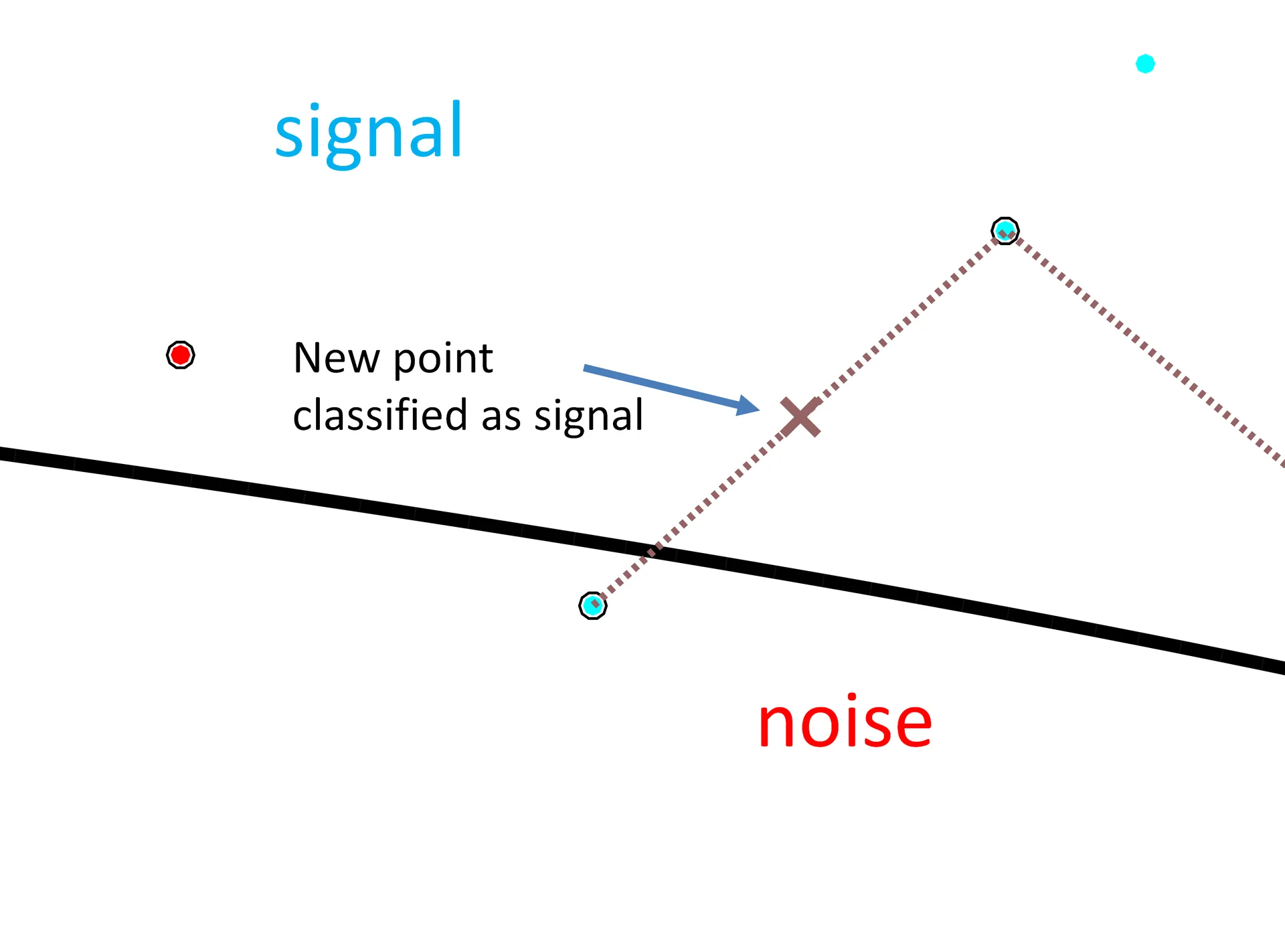
This resulted in two clear issues with this method. For one, since test error is a ratio of misclassified points to total points, if the algorithm misclassified none of the training data, this method would report a test error of 0, giving the researcher a false sense of the classifier’s efficacy. The second issue is that the set of data to be tested on has only the same number of elements as the number of points the algorithm. As such, the denominator of the test error ratio is small, leading to inflated rates of test error.
For the graph on the left, the orange line is the resulting test error curve for this method. This graph is simply the algorithm’s tune and test error rates (ratios) as a function of its complexity. In short, the blue line at the bottom of the graph is the true test error curve; which is what this line is supposed to look like.
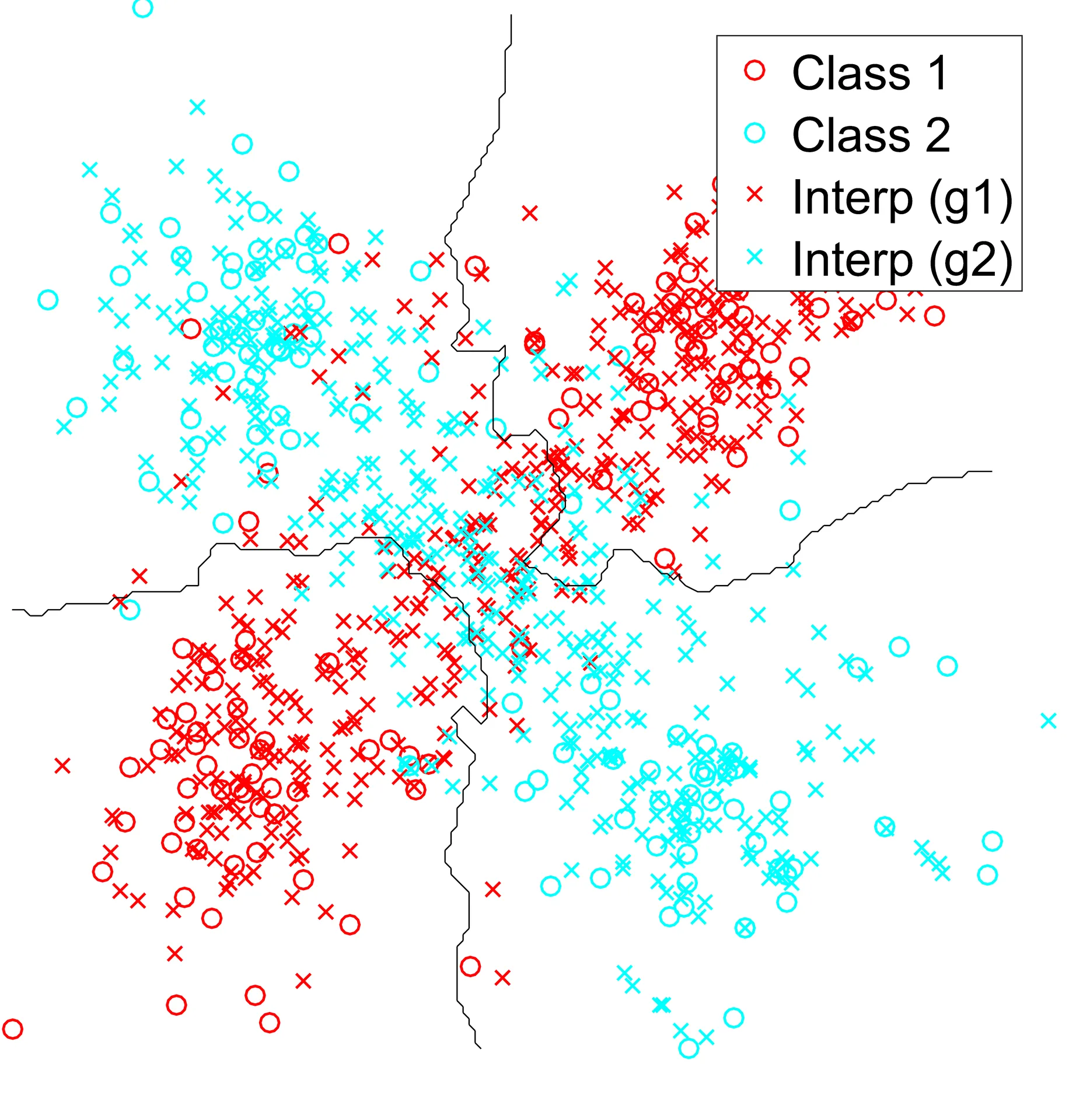
Naturally, I tried a different method. This time, I wanted to see what this test error curve looked like if I generated a test set by the following method: pair every data-point in each class with a different, randomly chosen point of the same class. Find a point that lies on the same line as these two points, and throw the resulting point into the test set with the same class label as the points from which it came. For a simple distribution, here is what that looks like for one class.
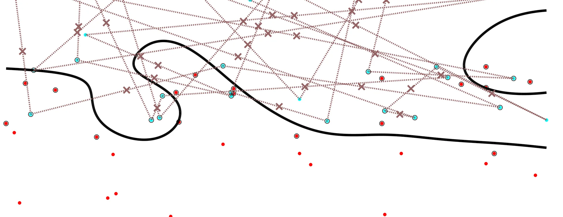 (image 9 of 19, view larger)
 (image 10 of 19, view larger)
I also tried fitting probability distributions to determine where along the line of interpolation or extrapolation that the new point landed, but to little avail. For various reasons, these interpolation schemes worked out quite poorly. A clear instance of linear interpolation failing was in a test case which I called the XOR problem; data that, as it sits in Euclidean space, is neighbored by large clusters of data belonging to the opposite class. Since these methods relied on interpolation between random pairs of data points, the resulting point often sat clearly in a cluster belonging to a different class.
Perhaps an even more important cause for failure was one that I took some time to stumble upon: what does any of this new data being generated have to do with the sample data? What does linear interpolation or extrapolation between random points have to do with the true distribution of the sample points? The answer, really, is that it doesn’t. Not even close.
In my frustration, I was led to a somewhat infantile question. If one line was not doing the trick, why not draw more? Could using the placement in Euclidean space of multiple points in relation to one another have a more beneficial affect? Though it was more difficult to come across, the answer this time was yes.
 (image 11 of 19, view larger)
The Final Solution
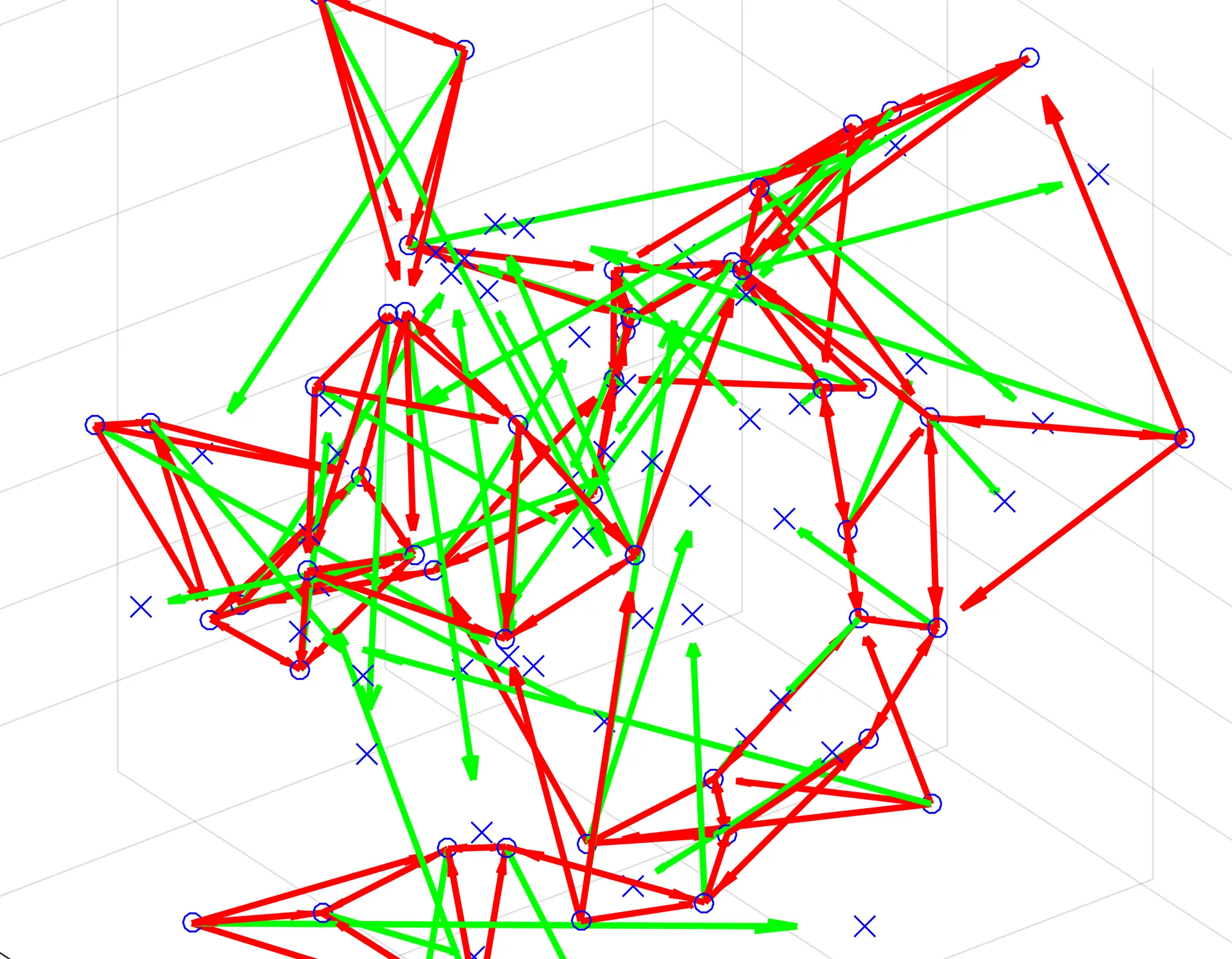
The final solution I came up with has many advantageous characteristics. To start, the algorithmic process is as follows.
- For each data point in every “class” of your sample data, identify the closest N nearest neighbors in Euclidean space.
- Create vectors {v1, v2, v3 … vn} from this point to each of its closest N neighbors.
- Note: N is the most variable parameter in this algorithm. I found that for large datasets with relatively few large clusters, round(sqrt(N)) is the optimal choice of neighbors. For most other cases, including real data and test cases that I generated, the optimal choice of neighbors is 4.
- Create a vector, R, which is the vector resulting from the component sum of the vectors
- Plot a new point at the head of R, and add this point to the test set
- Feed the test set into the trained classifier to return a quantitative measure of test error
This algorithm takes advantage of the relative density (read: clustering) of neighboring points in Euclidean space; a key component in ensuring that the new points are relevant to the original data distribution. This method also produces the same number of test points as there were points to train on, resolving the issue mentioned earlier of having too few or too many total points in the denominator of the test error ratio. On
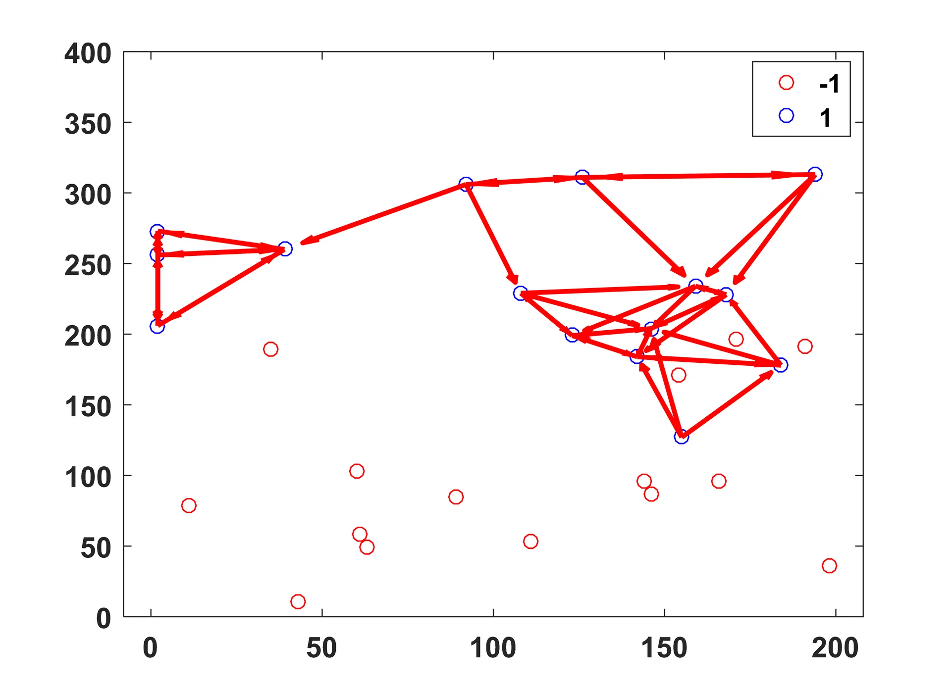
The spatial intuition for this method is as follows (choosing 3 nearest neighbors):
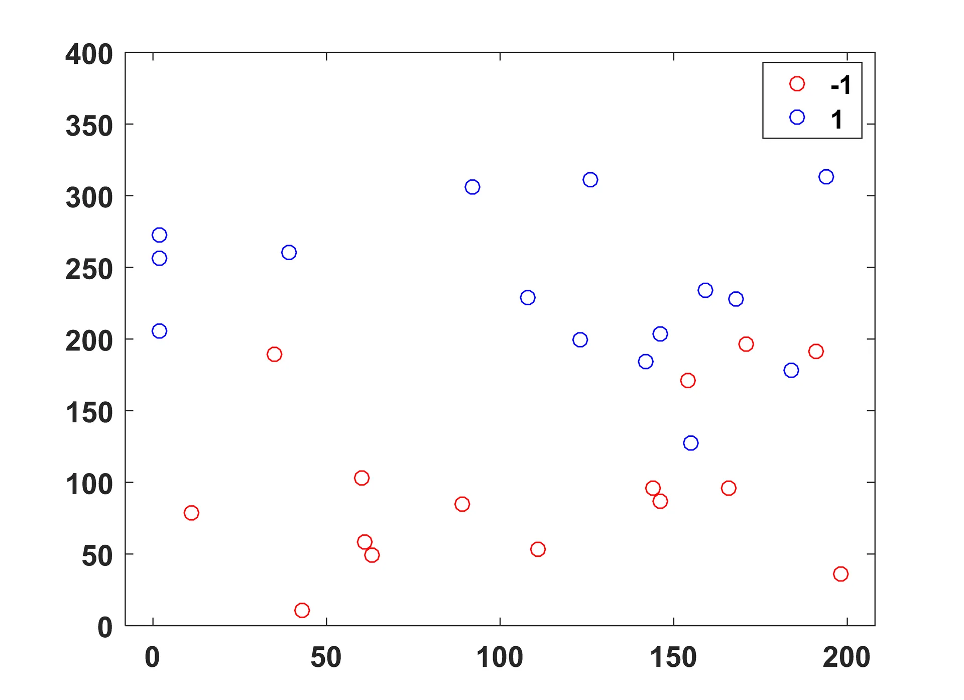
Sample points, as they sit in 2D Euclidean space.
Shown for one class, the nearest neighbor vectors are drawn in red.
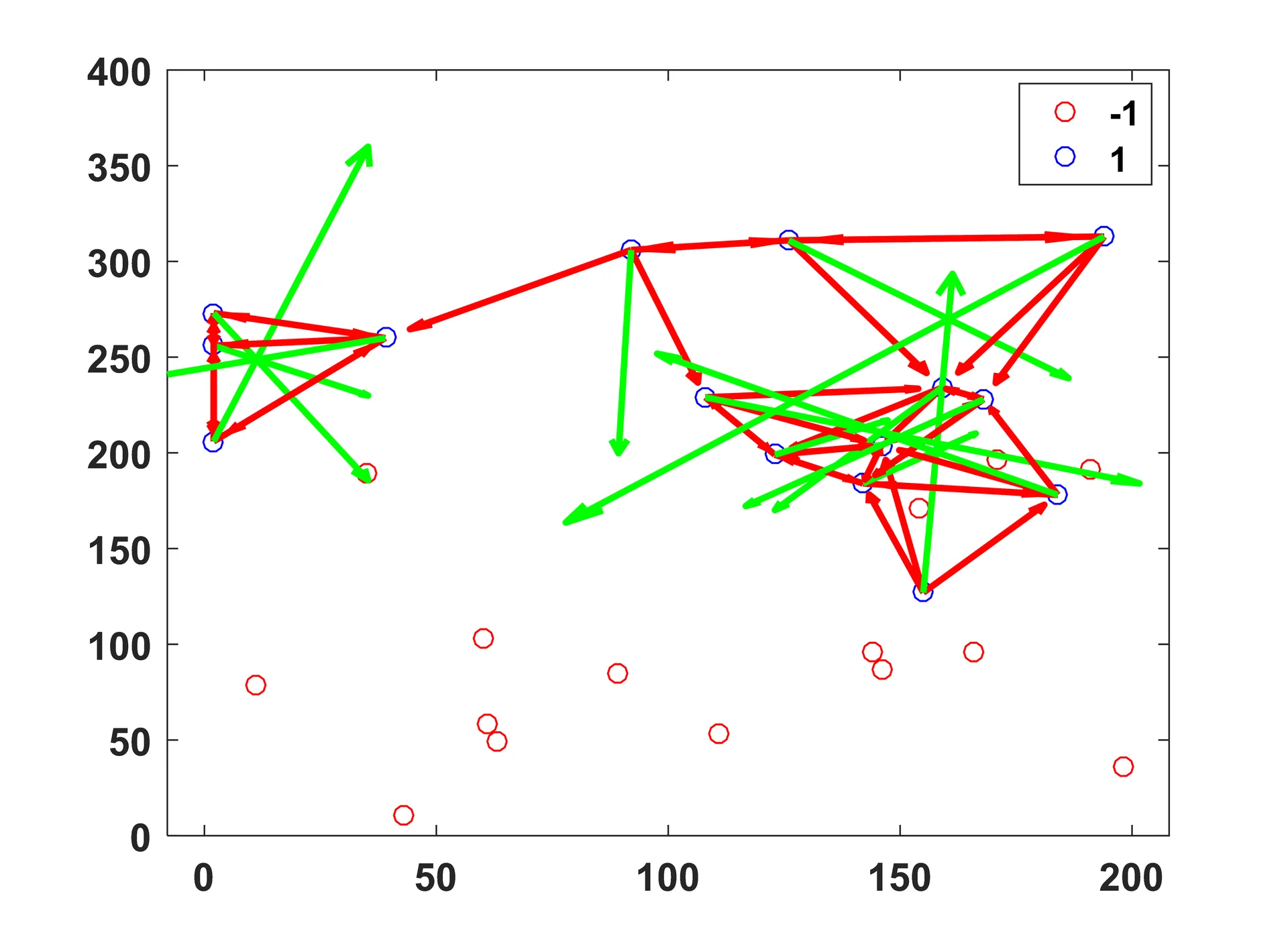
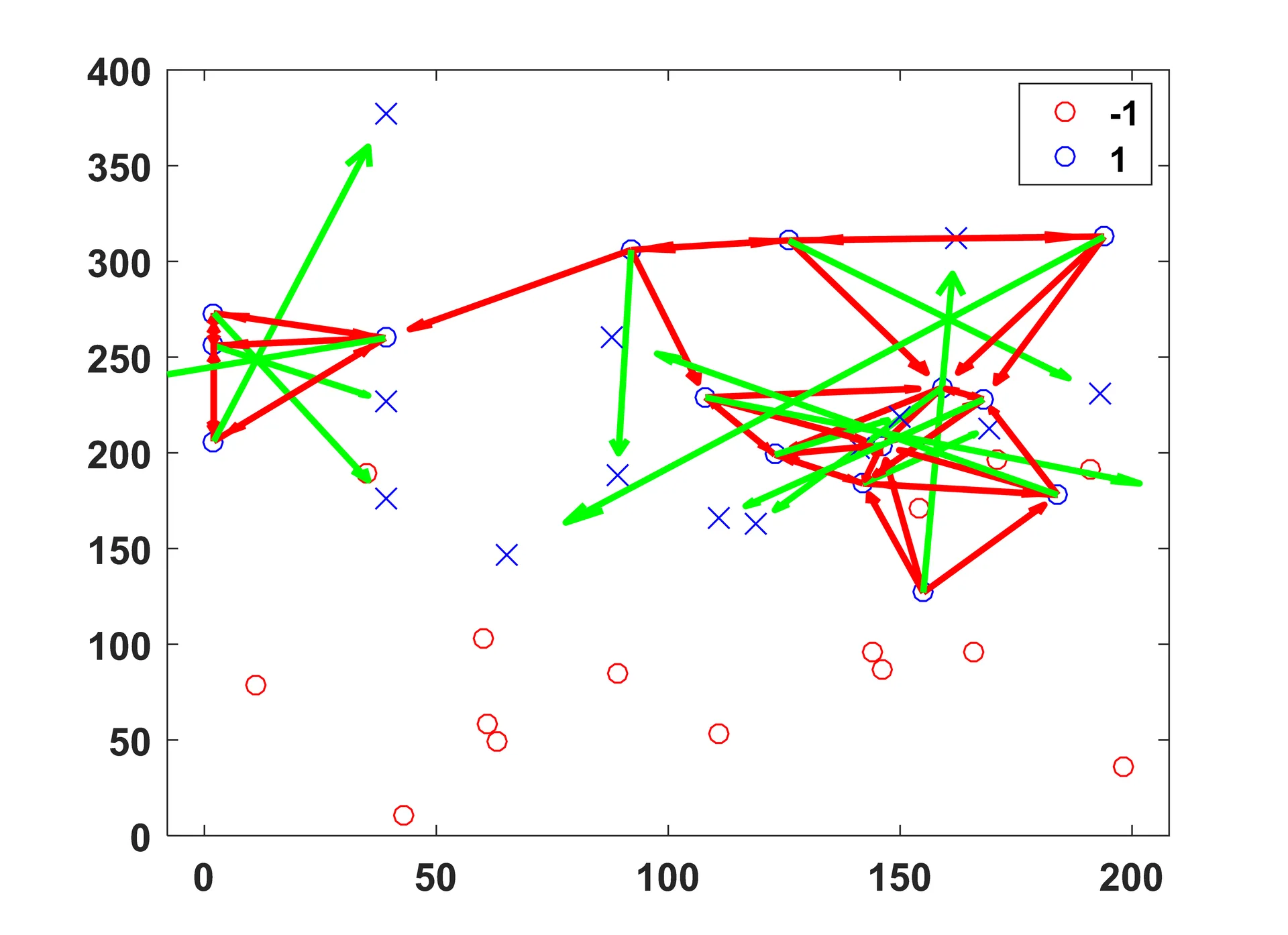
The component sum of these vectors, R, shown in green, is determined for each point.
The new data lies at the head of each resulting vector.
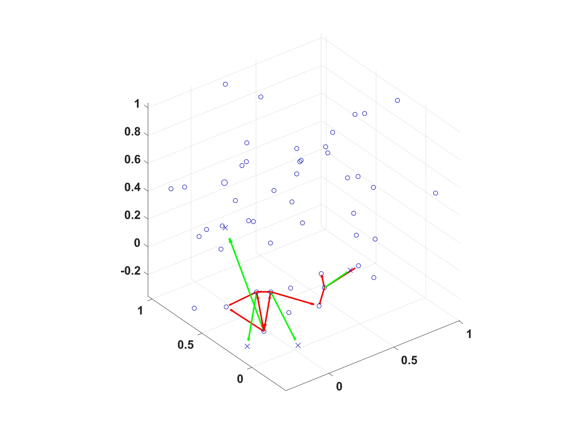
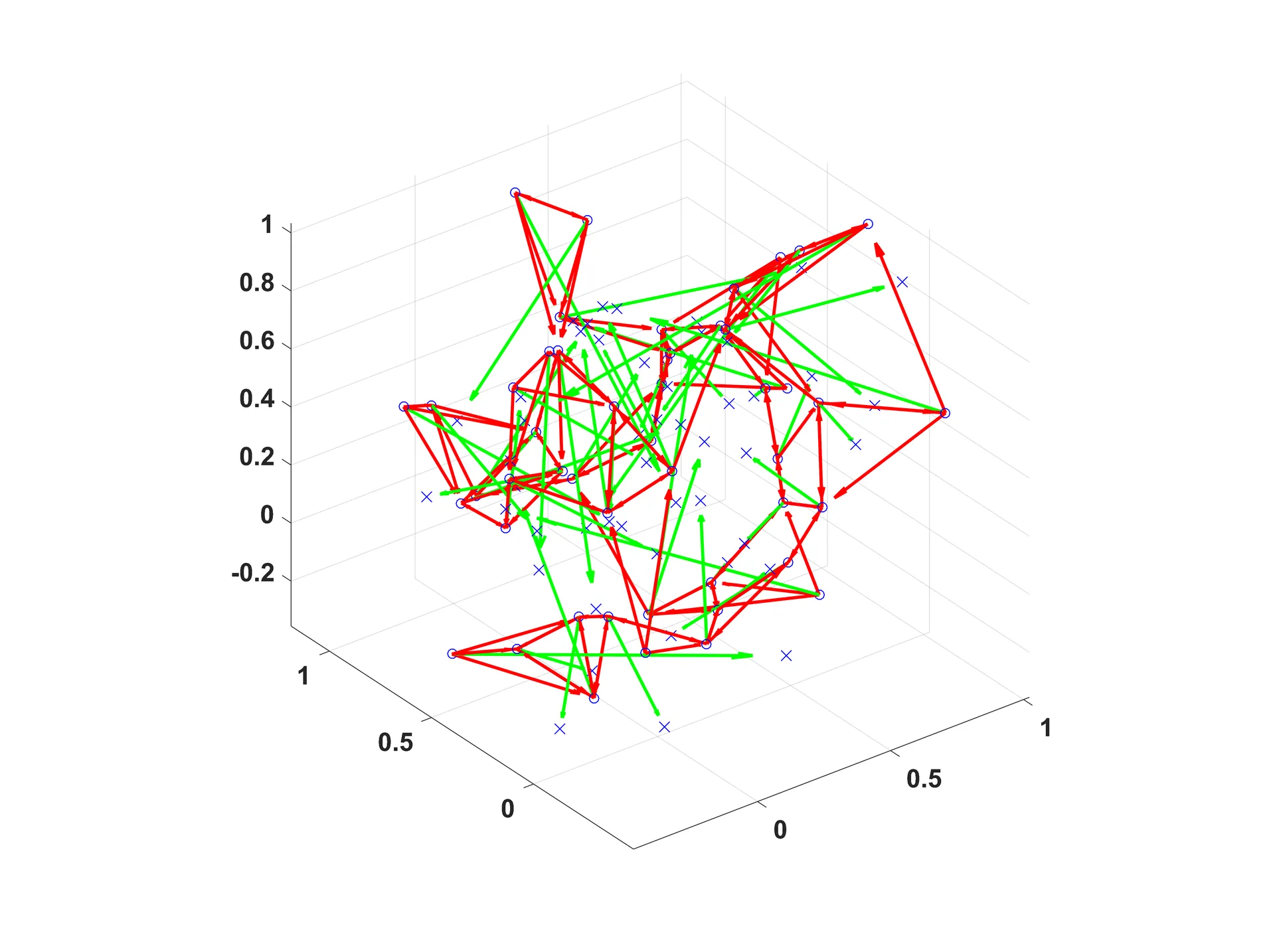
IN 3D
Testing the Algorithm
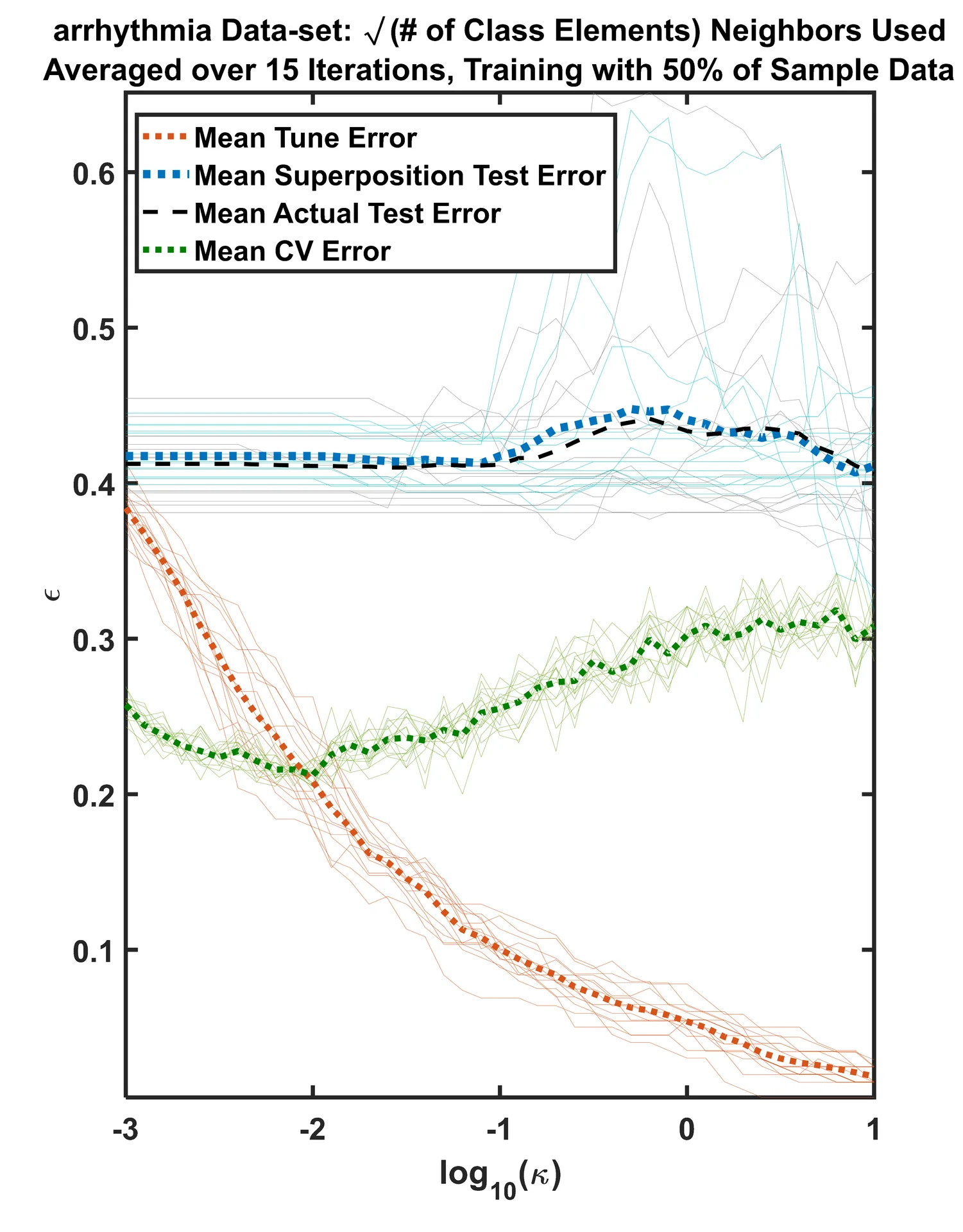
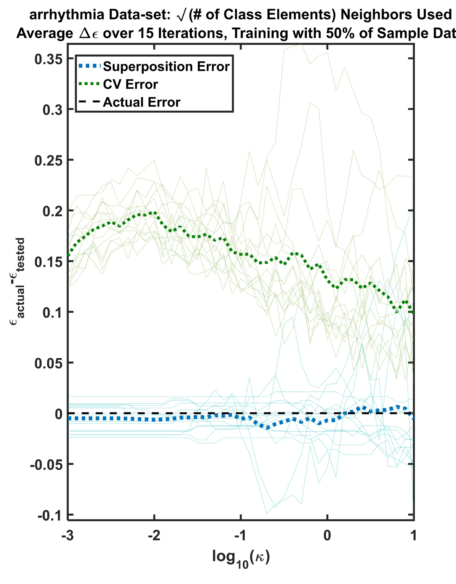
For an exhaustive list of test cases, my algorithm performed exceptionally. The biggest issues yet to solve are its time complexity [O(n2)], and a robust rationale for choosing how many nearest neighbors to consider. When the algorithm was tested on a Support Vector Machine classifier, trained on real data, the following tune vs. test errors were produced. What is most relevant is how close the blue line is (my algorithm’s error) to the black line (actual error), and how cross-validation, in this particular case, misjudges the algorithm’s test error. On the right is the difference between the actual error and what the algorithm’s reported. Naturally, the closer to 0 each line on the graph resides, the better it was in estimation of the true test error.